How Do Neural Networks Learn

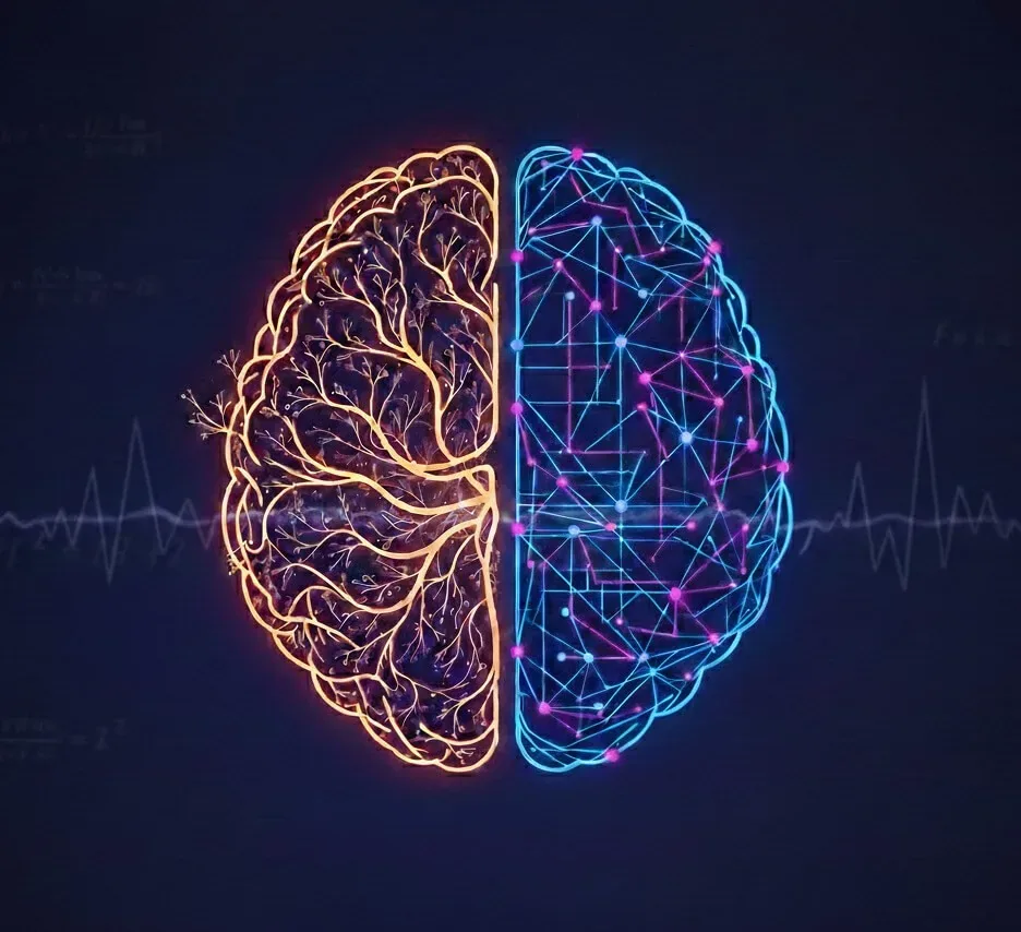
According to the National Library of Medicine, your brain has roughly 61 to 99 billion neurons, with each one firing signals thousands of times a second. An artificial neural network borrows that exact concept and runs it using straightforward arithmetic.

In this guide, we will break down how neural networks work, how they learn, and why something built from basic math can power systems that see, read, and understand our world.

---

The Brain, Simplified

Before moving forward, let's clarify what we mean by "the brain." At its core, our brain is a massive web of neurons, or brain cells, linked together so that every cell connects to many others.

Fun fact: In the time it took you to read this sentence, each neuron in your brain fired dozens of times.

Zoom in on a single biological neuron, and you will find it is remarkably simple.

A single neuron receives an input signal called a stimulus. If that signal crosses a specific threshold, the neuron fires. That is the whole story. A single neuron does not think, understand, or make complex choices on its own. It simply responds with a binary yes or no.

So how do billions of these simple units create thoughts, language, creativity, and decisions? The answer lies not in any individual neuron, but in the pattern of connections between them.

Let's look at a small example to see this in action.

A Tiny Network, A Real Insight

Imagine a network of just 5 neurons, where neurons 1 and 2 connect to neurons 3 and 4, which then send their output to neuron 5:

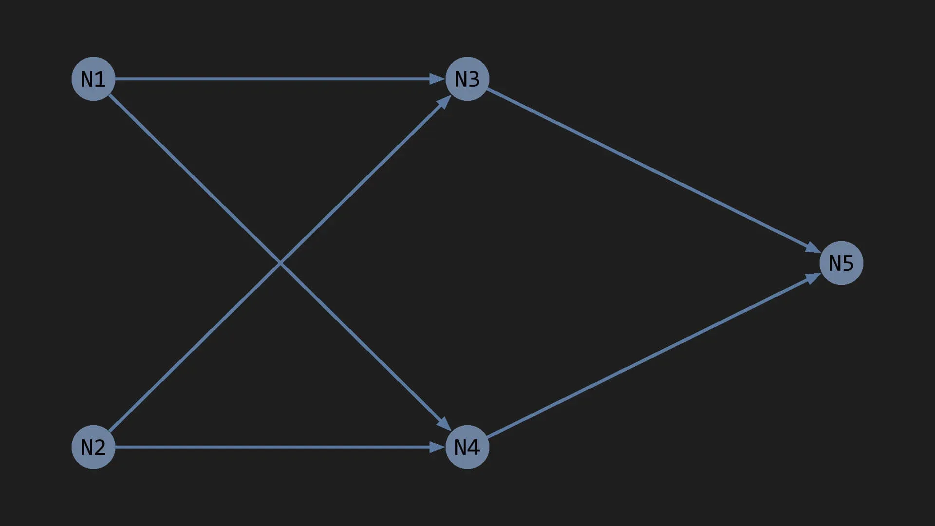
Here is the specific job for each neuron:

• N1: Fires when it detects eyes.
• N2: Fires when it detects a smile.
• N3: Fires when both N1 and N2 fire.
• N4: Fires when either N1 or N2 fires, but not both.
• N5: Fires only when N3 fires and N4 stays silent, signaling "happy face detected."

These rules are simple, but watch what happens when we run an input through them.

Let's test a happy face: 😀

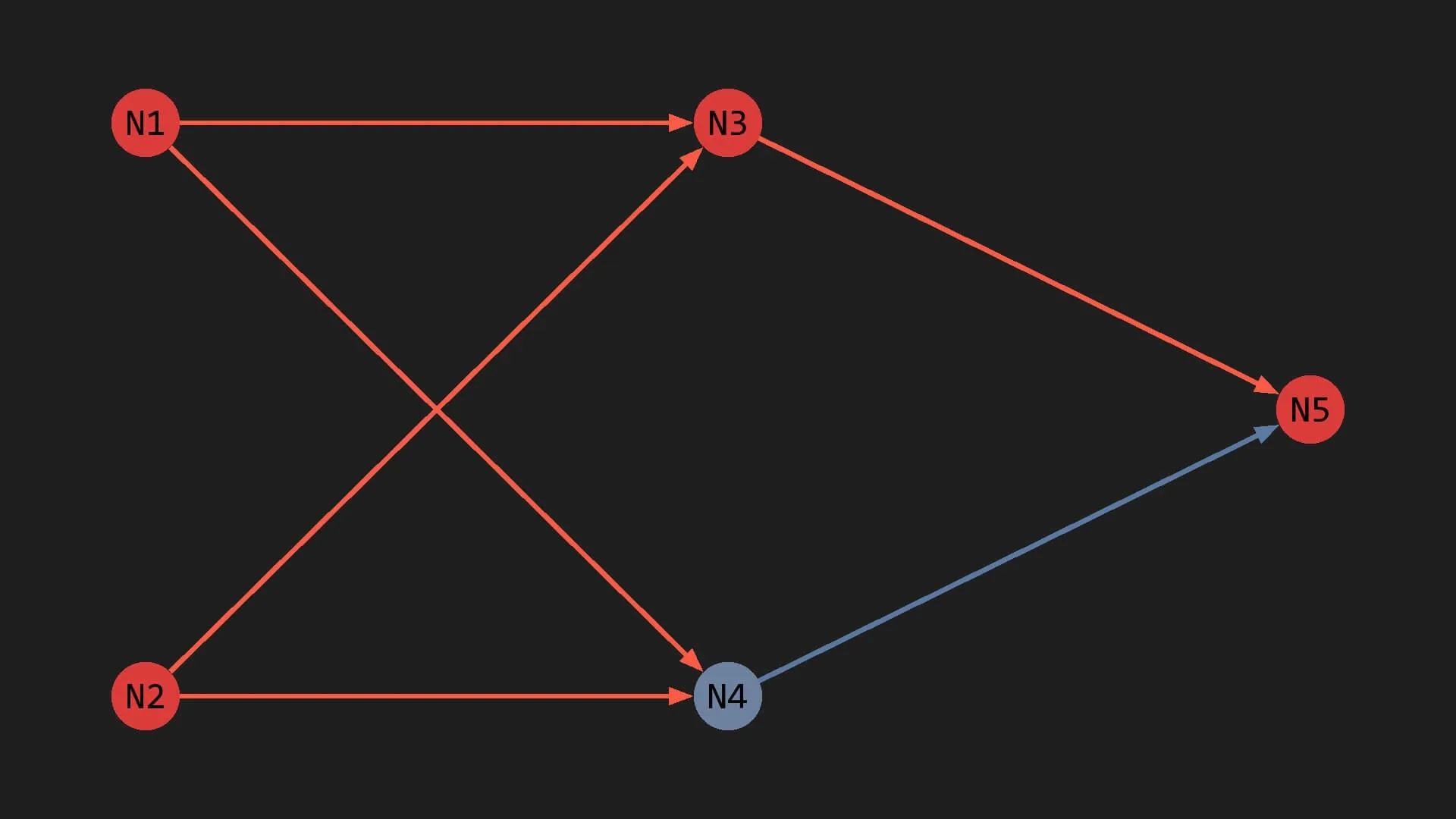
• N1 detects eyes and fires.
• N2 detects a smile and fires.
• N3 sees both N1 and N2 firing, so it fires.
• N4 stays silent.
• N5 sees N3 active and N4 quiet, so it fires.

The Result: N5 fires, confirming a happy face ✓.

Now let's test a sad face: ☹️

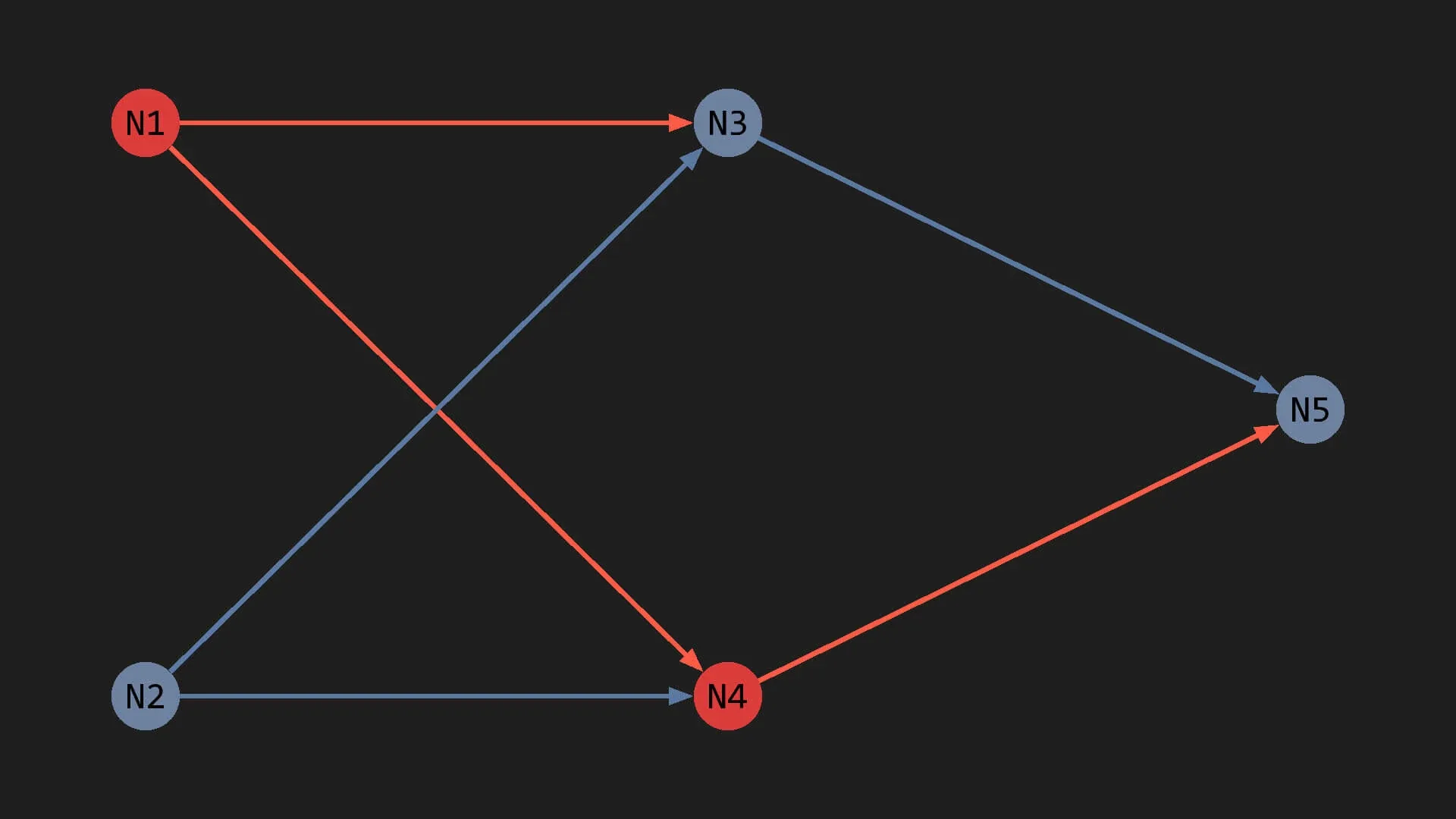
• N1 detects eyes and fires.
• N2 detects a frown and stays silent.
• N3 receives only one signal, so it stays silent.
• N4 receives only N1's signal, so it fires.
• N5 sees N3 is silent, so it stays silent.

The Result: N5 does not fire, indicating this is not a happy face ✓.

In both cases, each neuron followed its simple rule. None of them understand what a face or an emotion is. Yet through structured connections, clear logical patterns emerge.

This is how biological brains function, just scaled up significantly. When we break the concept into clear components, the math becomes far easier to follow.

Note: Real neurons do not directly identify eyes or smiles. Sensory organs translate physical inputs into electrical impulses, which neurons then process. This example is simplified to highlight the core structure.

The Three Building Blocks: From Biology to Math

To rebuild this system artificially, we swap biological cells for mathematical functions, and physical synapses for weighted links.
Here is how those core components map over:

1. The Activation Value (The Strength of the Signal)

Biological neurons do not operate purely as binary switches. They fire at varying intensities depending on the incoming stimulus.

We mirror this behavior by assigning every artificial neuron an intensity score between 0 and 1, called its activation value. A value of 0 means completely silent, 1 means firing at full capacity, and numbers in between reflect varying signal strengths.

It looks like this:

2. The Weight (Connection Strength)

Neurons rely on incoming signals from their neighbors. Some links carry strong influence, while others carry very little.

We model this influence by assigning each connection a numeric weight. A high weight means the incoming signal heavily drives the next neuron's activation. A lower weight means the signal barely alters the outcome.

In biology, some connections actively suppress downstream activity. This is known as inhibition. In artificial networks, we replicate this by allowing weights to be negative numbers.

3. The Bias (The Baseline Threshold)

If a neuron relied entirely on its inputs, a zero signal would always result in a zero output. To give neurons flexibility, we introduce a baseline tendency to fire or remain quiet regardless of input.

We call this value the bias. It is an offset added directly to the total signal, giving each neuron an independent threshold.

Putting It All Together

Combining activations, weights, and biases gives us the core calculation for a single connection: bias + (activation * weight)

Every artificial neuron runs this exact operation.

When a neuron receives inputs from multiple sources simultaneously, it sums their combined values before applying its bias.
Try visualizing how these signals sum up before moving to the example below.

Consider a setup where neuron N3 has a bias of 0.10, receiving signals from N1 and N2 at the same time.
N3 combines these inputs through addition:

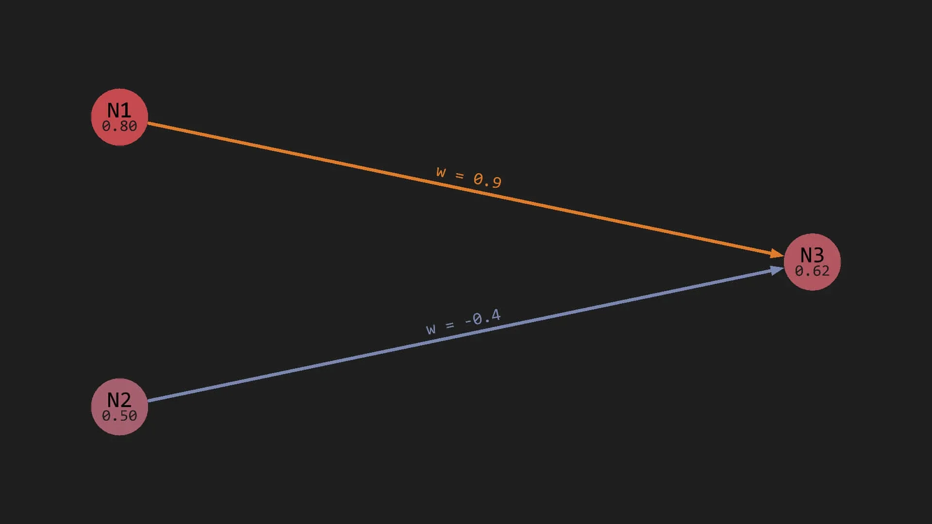
N3 activation = (N1 activation * weight to N3) + (N2 activation * weight to N3) + N3 bias

Plugging in the numbers gives: 0.8 * 0.9 + 0.5 * -0.4 + 0.1 = 0.62

That simple arithmetic runs millions of times across connected layers.

The Activation Function: Keeping Signals Bound

In our example, N3 produced an activation of 0.62. But without boundaries, repeated multiplication and addition could yield values like 15.4 or -8.2.

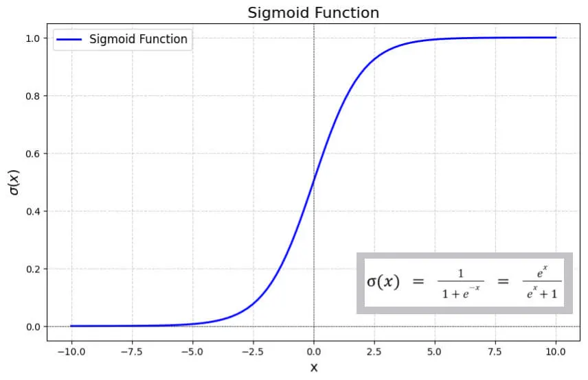
Unchecked numbers quickly destabilize a network as signals cascade through deep layers. To keep activations manageable, we pass the result through an activation function that squashes raw totals back into a strict range like 0 to 1.

One classic choice for this step is the sigmoid function, which maps any input number smoothly onto a scale between 0 and 1.

How Networks Learn

This is where static equations turn into adaptive systems.

When a network is first created, its weights and biases are filled with random numbers. Asking an untrained network to classify an image will yield random guesses. It might look at a photo of a dog and output a high confidence for a sailboat.

Because setting millions of parameters manually is impossible, we use a feedback loop: predict, measure the error, and adjust the weights.

The training cycle follows these core steps:

• Feed labeled data into the input layer.
• Calculate the network's final output.
• Compare that output to the correct target to calculate the error score.
• Determine how much each specific weight and bias contributed to that error.
• Apply a small numerical adjustment to nudge parameters closer to the correct answer.

We adjust parameters gradually. Large changes ruin overall stability, so every weight receives a slight shift proportional to its responsibility for the mistake.

Repeating this loop across thousands of examples gradually shifts random values into precise parameters tuned for specific tasks.

This iterative tuning process is called training. The capability of modern AI stems directly from repeating this simple update loop at massive scale.

To trace how error values travel backward to update individual parameters across deep layers, we use an algorithm called backpropagation.

Backpropagation is the core engine behind modern neural networks. To see how the underlying calculus handles these updates step by step, read our full breakdown here: Backpropagation: How a neural network learns from its mistakes.

Layers: Organizing Complex Inputs

Connecting every neuron to every other neuron becomes computationally impossible as networks grow. Five neurons require 20 directed links, while 1,000 neurons would require nearly a million connections. We need systematic organization.

We solve this by arranging neurons into distinct layers. Information flows sequentially from one layer to the next, converting complex webs into predictable pipelines.

Note: While biological brains use complex interconnected circuits, layered structures allow digital hardware to calculate updates efficiently.

Here is how information travels through layered arrangements:

Standard networks split their structure into three layer roles:

• Input Layer: Receives raw external data. For images, each input neuron holds the normalized intensity value of a single pixel.
• Output Layer: Produces the final result. A digit classifier uses 10 output neurons, where each value represents confidence for numbers 0 through 9.
• Hidden Layers: Intermediate steps where features are extracted and combined. Deep architectures stack multiple hidden layers to recognize complex patterns.

Seeing the Math in Motion

The graphic above shows a real network updating its parameters in real time. Starting from random initializations, systematic updates shape raw weights into functional decision boundaries.

At every step, the underlying arithmetic remains identical: multiply inputs by weights, add biases, apply an activation function, and adjust parameters based on error.

By combining these elementary building blocks across large layer architectures, networks learn to process visual data, analyze text, and recognize audio patterns directly from data.

Research continues into optimizing these architectures, balancing theoretical models with empirical performance across complex real-world tasks.

As these architectures expand, they offer practical tools for pattern recognition and automated analysis across every major domain.

---