Backpropagation: How a Neural Network Learns From Its Mistakes

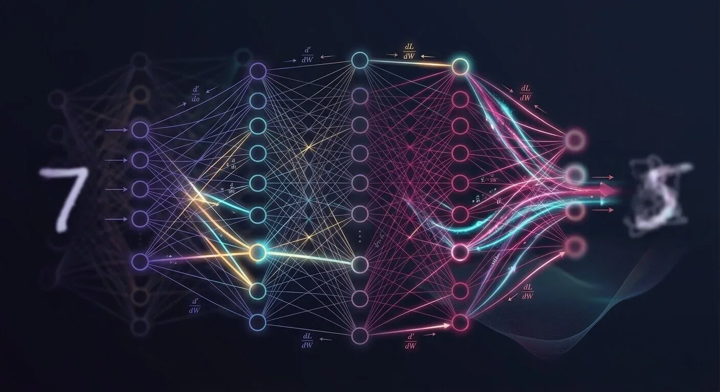
Your brain has never read a textbook on how to recognize faces. Yet you can glance at a stranger across a crowded room and instantly know: that's a person, that's a smile, that's someone you haven't met before. No one programmed that in. You just learned it.

Artificial neural networks learn the exact same way. Not through hand-written rules, but through constant repetition and real-time corrections. Show the network enough examples. Tell it when it gets something wrong. Let it adjust its internal knobs, then repeat the process.

The underlying engine making those updates possible (the actual mechanism that drives learning) is called backpropagation. In this guide, we will break down how it works step-by-step in plain, beginner-friendly language.

Recap

If you've already read our introduction to neural networks, you know the basic setup: a grid of artificial neurons holding numbers, connected by weights and biases, processing signals layer-by-layer until an answer pops out the other end.

If that's new to you, don't worry! Everything you need to follow along will be explained right here. But if you want to build the full foundation first, this guide covers the basics from scratch: How Do Neural Networks Learn?

At the heart of machine learning lies a simple, slightly uncomfortable reality. When a neural network is first initialized, every weight and bias inside it is just a random guess. The system has zero built-in logic, intuition, or context. Ask it to read a handwritten digit and it might look at a sharp, clear 7 and confidently call it a 2. It isn't being careless; it genuinely has no idea what it is looking at yet.

So, how do you transform a massive collection of random numbers into a smart, reliable model?

You correct it the same way you would fix any real-world mistake: figure out what went wrong, trace the error back to its source, and make an adjustment. Then run that loop thousands of times over.

That is backpropagation in a nutshell. It isn't magic or synthetic intuition. It is a systematic, mathematical audit asking: Which parts of the network caused this mistake? From there, it makes sure every component makes a slight correction to prevent that error next time.

The core idea is straightforward. Sending information forward through a network is easy: input comes in, math happens across each layer, and a prediction comes out. But true learning happens in reverse. We take the incorrect prediction, walk backward through every layer, and pinpoint exactly how much each weight and bias pushed the answer off course. That shows us which direction those values need to shift for the next run.

This reverse pass is what gives backpropagation its name. By the end of this guide, you will be able to follow every single step of that journey.

Measuring The Mistake

Before we can fix a network's output, we need a precise measurement of how wrong it actually is. We cannot use general feedback; we need a concrete number we can calculate, track, and systematically reduce over time.

This brings us to the loss function. You can think of loss as a penalty score: the lower the number, the better the performance.

Once the network produces a prediction, the loss function compares that output against the true label from our dataset and outputs a single score representing the mistake. A loss score of zero means the network got it completely right. A higher score points to a bad prediction, with larger numbers highlighting bigger misses.

Let's walk through a concrete example to see this in practice:

Suppose we are training a network to recognize handwritten digits. We feed it an image of a 7. The network outputs a confidence score for every number from 0 through 9, showing how strongly it believes the image matches each digit. In an ideal setup, the raw predictions would look like this:

0

0

0

0

0

0

0

0

0

However, an untrained network operating on random weights might give us chaotic outputs like this instead:

0.3

0.2

0.9

1.0

0.3

0.5

0.1

0.1

0.6

Note: These numbers are completely arbitrary sample values used to demonstrate the main concept.

This output is clearly off target. But simply saying it is "wrong" does not give our math anything to work with. We need to measure that error numerically.

Our immediate instinct might be to calculate the simple difference between the network's guess and the correct answer for each slot, then sum them up. While that works, practical machine learning relies on a smarter alternative: squaring those individual differences instead of using raw subtraction.

Why does squaring make such a difference?
For the digit 7, we expected 1.0 but got 0.1. The raw difference is 0.9, which squares to 0.81 (still a major error).
For the digit 5, we expected 0.0 but got 0.3. The raw difference is 0.3, which squares down to a tiny 0.09.

Squaring changes how the network views its mistakes. It magnifies massive blunders while minimizing small, acceptable variations. A model that makes a huge, overly confident mistake on one item gets penalized far more than one that is just slightly off across several spots. That is precisely how we want our model to adjust, since large, confident errors cause the most issues.

When we average all these squared differences across every output option, we get our single error score: the Mean Squared Error.

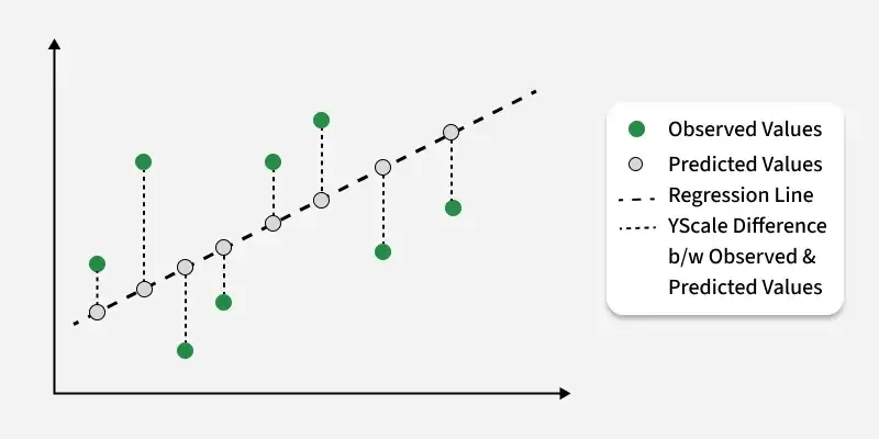
With Mean Squared Error in place, we now have a clear target score: our loss. The main goal from here is simple: nudge each weight and bias in the right direction, by the right amount, to pull that loss score down.

The Right Direction

We now have a clean metric showing how far off our model's predictions are, and we know we want to push that number down. But modern neural networks contain thousands (or even millions) of internal parameters. Think of every weight and bias as an adjustable dial. Turning any single dial alters the final loss, but how do we know which dials to turn and which way to spin them?

If you adjust a weight slightly and the overall loss goes up, you moved in the wrong direction. If you adjust it the other way and the loss drops, you found the right path. Testing every dial through trial and error would take forever, so we need a systematic way to calculate the best shift for all parameters at once.

This optimization strategy is known as gradient descent.

Picture your network's overall loss as a vast, hilly landscape full of peaks and valleys. Every unique combination of weights and biases places you at a specific spot on that terrain, where the altitude represents your current loss score. Our goal is to walk down into the lowest possible valley.

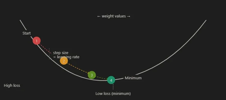
The gradient simply measures the slope of the ground right under your feet. It points straight uphill toward higher loss. Because we want to minimize error, we take a step in the exact opposite direction (downhill), evaluate the slope at our new position, and take another step forward.

Each step represents an update to our internal parameters. How big should that step be? That is determined by the learning rate parameter. Setting the learning rate too high causes the model to jump over valleys and bounce off walls endlessly. Setting it too low makes training painfully slow and computationally expensive.

Here is the catch: calculating the slope tells us where downhill lies, but it doesn't automatically show how much every individual weight contributed to our current position. We cannot manually tweak millions of weights one by one to see what happens. We need a way to map that overall slope back to every parameter in a single pass.

That exact step is where backpropagation comes into play.

A helpful distinction: gradient descent is our overall strategy (finding the downhill path and walking toward it). Backpropagation is the underlying mechanism that makes gradient descent practical at scale. It carries out the calculus needed to reveal which way is downhill for every single weight inside the network.
They are distinct tools that function as a team: gradient descent picks the direction, while backpropagation does the math required to guide those steps.

Tracing the Blame

Let's look at a core challenge in training these models:

The network made a mistake, and the loss score tells us how severe it was. But that score sits at the very end of our system, while the weights driving the mistake are spread across every layer. How do we measure the exact portion of blame belonging to each individual parameter?

The answer is to work backward, one layer at a time.

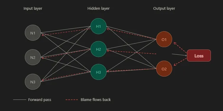
Consider how the network calculated its final output in the first place. Neurons in the output layer fired based on signals from the hidden layer, which originally picked up signals from the input layer. Every node across the entire network played a role in the final answer. The question now is: how big was each node's impact?

We start at the finish line, right next to our loss score. The output neurons have the most direct link to the mistake. Because our loss calculation follows a strict mathematical formula, we can take its derivative with respect to each output node. That derivative tells us whether increasing a specific output node pushes the loss up or down, and by how much.

Next, we step back one layer. The nodes in our hidden layer generated the values that our output layer acted on. So we ask a similar question: if a hidden node's value shifts slightly, how does that alter the output layer, and how does that shift trickle down to affect the overall loss?

We repeat this exact step all the way back to the initial input layer. At every step along the way, we ask one focused question: If this internal value changes slightly, how does that ripple downstream? We then multiply those local impacts together as we trace backward.

The Chain Rule

That backward multiplication relies on a fundamental mathematical tool: the chain rule.

If input A impacts value B, and value B impacts outcome C, then any small change in A trickles through to C via B. The chain rule in calculus gives us a direct formula to compute that full relationship: the rate at which A changes C equals the rate at which A changes B, multiplied by the rate at which B changes C.

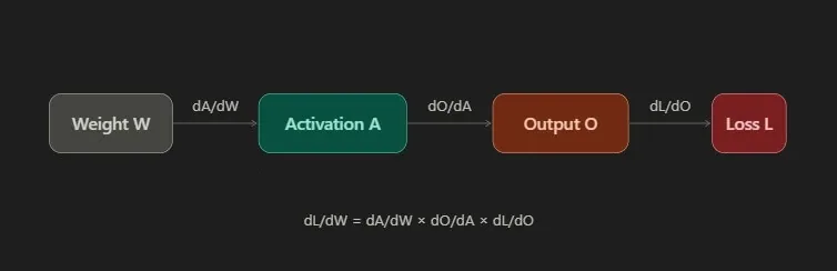
Inside a neural network, that chain of events looks like this: weight → node activation → next layer activation → output prediction → final loss. Backpropagation steps through this chain in reverse. At each layer, it computes local derivatives to see how those values impact the next step. It multiplies those rates together to calculate the complete gradient, showing how much a weight near the input layer drives the final error.

This approach keeps the training process fast and practical. Instead of running millions of separate tests for every parameter, you complete a single backward pass through the network, reusing shared calculations along the way. Computing these gradients for the entire model takes roughly the same time as running a standard forward prediction.

Updating the Weights

Once we compute the gradient for every weight and bias, we hold two key pieces of information: which direction increases the error (uphill), and which direction reduces it (downhill). From there, we adjust every parameter one small step toward the downhill path.

The standard update formula looks like this:

        Updated weight = current weight - learning rate * gradient
      

In simple terms: your new weight equals the old weight minus a small step in the direction of the gradient. The learning rate term controls how far we step during each update. The gradient calculation tells us how much that specific weight contributed to the error and which way it pushed the result.

A positive gradient means increasing the weight drives the loss higher, so we subtract to nudge the weight lower. A negative gradient means the weight was already pushing loss down, so subtracting a negative value nudges it further in that helpful direction. In both cases, the overall loss drops slightly after the update.

Then we repeat the loop. Feed the network another example, run the forward pass, calculate the loss, run backpropagation, and update every parameter. Do this across thousands of training examples, and those initial random guesses slowly transform into precise, reliable values that work.

Putting It All Together

Let's zoom out and look at the complete training process.

A neural network begins as a collection of random weights and biases, completely unable to perform useful work. We pass a training sample forward through the network layer-by-layer until it generates a prediction, then measure how far off that prediction was using a loss function. Next, backpropagation runs in reverse, passing the blame backward through every layer using the chain rule to calculate each weight's exact contribution to the error. Gradient descent uses those gradients to shift every weight one step closer to lower error, and the entire cycle repeats.

What makes this system remarkable is how simple the individual steps are. The forward pass relies on basic arithmetic, the loss score comes down to simple subtraction and squaring, the chain rule is standard calculus, and the weight update is basic algebra. Yet when you chain these simple operations together across millions of cycles, the model begins discovering deep structural patterns on its own. A network that started out unable to distinguish a 7 from a 2 learns to read handwriting with incredible precision, not because it was given explicit rules, but because the math guided it there.

Backpropagation is not conscious thought or human-like understanding. At its core, it is simply an efficient method for answering one question: Which parts caused this error? By making tiny, continuous adjustments based on that answer, genuine task intelligence naturally emerges over time.

The next time you ask an AI model to identify an image, translate text, or draft an email, this exact processing loop is running under the hood. Millions of forward passes, millions of backward adjustments, and millions of tiny weight updates all working together until the math clicks into place.

---